Capture ratio — wind cannibalises its own price
Capture-price ratio (capture price / time-weighted wholesale) falls over time as wind capacity grows. The AR1 wind CfD levy rises in lockstep — the two lines are mirror images of the same mechanism.
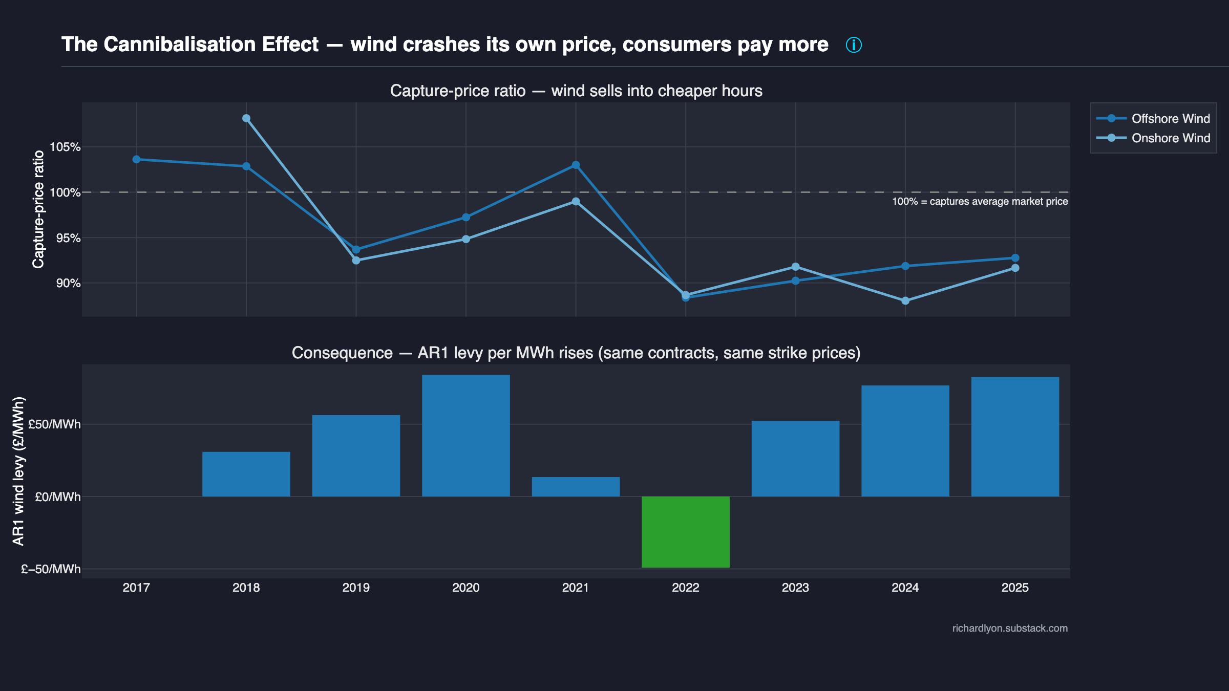
What the chart shows
A two-panel diagnostic with a shared x-axis (calendar year, scheme start to the most recent complete year).
Top panel — capture-price ratio. For each year and each technology (Offshore Wind in deep blue, Onshore Wind in light blue) the chart plots the capture-price ratio: the generation-weighted average wholesale price received while that technology was generating, divided by the unweighted time-weighted average of the same wholesale price. A ratio of 100% (marked with a grey dashed reference line) means the technology captured exactly the market average — its generating hours were representative. A ratio below 100% means the technology's output concentrated in hours when wholesale was cheaper than average — classic cannibalisation. Both wind lines trend downward over time.
Bottom panel — AR1 wind levy per MWh. A bar chart of the average
CfD levy payment per MWh for AR1 wind units: CFD_Payments_GBP /
CFD_Generation_MWh by year. Bars are colour-coded — blue for positive
levy (consumers topping up), green for negative (clawback, i.e.
generators paying consumers back during the 2022 gas crisis window).
The panel is restricted to AR1 wind because those units have stable,
long-dated strike prices: any change in levy-per-MWh over time is pure
market-side movement, not strike-price variation.
The argument
The more wind we build, the more it crashes its own price — and consumers top up the difference via CfD. Cannibalisation is self-inflicted and baked in.
Wind's output is fundamentally concentrated in high-wind hours. As the UK fleet grows, those high-wind hours become increasingly oversupplied, pulling the wholesale clearing price down at exactly the moments when wind is earning. The generation-weighted wholesale price (the "capture price") therefore drifts further and further below the unweighted time-weighted average: the capture-price ratio in the top panel falls.
The CfD mechanism exists precisely to guarantee the gap back to the generator. Strike price minus the market reference price is paid out of the Supplier Obligation levy on every consumer's electricity bill. So the falling capture price in the top panel must translate into the rising levy per MWh in the bottom panel — they are literally the same number presented two ways. You can read the mechanism working in real time: every percentage point the top-panel line drops shows up as extra pence on the bottom-panel bar.
This matters for any assessment of "does building more wind reduce consumer bills?" The wholesale saving is refunded to the CfD generator through the levy: the two effects cancel for CfD-contracted generation by design. What scale-up of wind delivers, under CfD, is a reallocation from wholesale to levy — plus a growing capture-price penalty that shows up specifically as rising levy.
Methodology
Source: LCCC Actual CfD Generation and avoided GHG emissions (daily
settlements with per-row Market_Reference_Price_GBP_Per_MWh,
Strike_Price_GBP_Per_MWh, CFD_Generation_MWh, Technology,
Allocation_round, and CFD_Payments_GBP).
Capture price for technology T in year Y, using LCCC's per-unit Market Reference Price (MRP):
capture_price(T, Y) = sum(MRP_row × CFD_Generation_row)
                    / sum(CFD_Generation_row)
                    for rows where Technology = T and year = Y
Time-weighted wholesale for year Y:
daily_mrp(d)     = mean(MRP_row for all rows on day d)
time_weighted(Y) = mean(daily_mrp(d) for all days d in Y)
Capture-price ratio: capture_price(T, Y) / time_weighted(Y) × 100.
A ratio below 100% indicates cannibalisation; values above 100%
indicate that the technology's generating hours priced above market
average (rare for wind; was briefly the case during early 2022 for
some offshore units).
Bottom panel — AR1 wind levy per MWh:
ar1_wind = df[Technology contains "Wind" and Allocation_round = AR1]
ar1_annual[Y] = sum(CFD_Payments_GBP) / sum(CFD_Generation_MWh)
                for rows in AR1 wind × year Y
AR1 wind is chosen because it has the longest stable-strike-price record.
Units filtered to CFD_Generation_MWh > 0 and to years with at least
10,000 MWh of generation to avoid pre-commissioning noise. The current
incomplete calendar year is excluded from both panels.
No gas counterfactual is used — this chart is a market-internal diagnostic: capture vs market, wholesale vs levy, all drawn from the LCCC dataset alone. See the Cannibalisation methodology for formal definitions of "capture price" and "time-weighted wholesale".
Caveats
- Wind-only technology filter. Solar is excluded from both panels because solar CfD units have too few CfD-exercising years (most strike-crossing only began in 2022+) for the same-diagnostic decomposition to stabilise. A solar capture-ratio panel can be added once AR3+ solar has 3+ full years of data.
- AR1 wind bottom panel is small-N. Only 22 AR1 wind units; aggregating annually gives one data point per year. Once AR2 and AR3 wind mature the bottom panel can decompose further by round.
- Dependence on LCCC's
Market_Reference_Price_GBP_Per_MWh. The capture-price ratio is driven entirely by LCCC's published MRP. If LCCC ever changes reference-price source (e.g. from N2EX day-ahead to balancing-market reference), the ratio shifts abruptly with no underlying physical change. The chart inherits LCCC's definition unaltered. - The time-weighted baseline is a proxy. Strictly, the "market average" a real-money generator might capture against is a system-weighted wholesale price across all generators. The chart uses LCCC's per-unit MRP as a daily proxy — close but not identical.
Data & code
- CfD data — LCCC Actual CfD Generation and avoided GHG emissions
- Chart source —
src/uk_subsidy_tracker/plotting/cannibalisation/capture_ratio.py - Tests —
tests/test_schemas.py(validates the LCCC Actual CfD Generation schema — this chart's entire input contract).
To reproduce:
See also
- Cannibalisation methodology — capture-price formula and definitions.
- Cost theme — the levy rise is the per-MWh component of the Cost theme's total £bn story.
- Generation heatmap — the concentrated high-wind hours cannibalising wholesale.
- Subsidy per tCO₂ — the economic diminishing-returns mirror.